Introduction to ACME
Welcome to the ACME user guide. ACME (ACoustic Measurement Environment) is a multi-purpose acoustic measurement and analysis tool. It provides tools for measuring, a signal generator, power spectra and sound level analysis.
Additionally, ACME is the required software for performing μZ impedance tube (product page) measurements and analyses. More information on the measurement and analysis procedures for this system can be found at the µZ impedance (user guide).
For more detailed description, please continue reading this user guide. This ACME user manual covers ACME version v0.8.x.
Reporting bugs
If you find any software bugs, inconsistencies, errors or improvement hints, please let us know on support@ascee.nl and we will fix it as soon as possible.
A privacy notice
We value your privacy, so we do not store unnessesary (personal) information. No (tracking) cookies are stored. We do a small bit of analytics for this site, just to see how many people are watching our documentation and to have a rough idea of where they are from1. Basically the only thing happening is a counter increase of the number of unique visitors we get.
Notes on this manual
The user interface of ACME picks up the style from its operating system. Therefore, colors, styles and places of buttons can vary a bit depending on your used operating system. There might be small differences between the screenshots in this user manual and the actual user interface.
We did our best to provide a proper manual, free of errors. However, if you do find an error or incomplete part, please let us know by sending an email to support@ascee.nl.
Enjoy!😄
-
This is done by masking the last byte of the IP address ↩
Overview of ACME
ACME's functionality is split into two major groups, called Measure and Analyze. As such, the software is split in two panels / tabs.
The Measure tab contains functionality for recording measurements, including a
signal generator and signal monitors. ACME measurements are stored in separate
files and are grouped together in a working folder. The measurements can be
inspected, processed and plotted on the Analyze tab.
important
An ACME session is tied to a folder on your system. When you start ACME,
we recommend to first select a proper folder where the measurements are to be stored.
This is done by clicking in the Menu bar: File->Open measurement folder..., or by > pressing the corresponding button on the toolbar.
Measure tab

The figure above shows an overview of the Measure tab.
- The DAQ configuration allows editing and configuring the DAQ devices. This
works using presets, which are stored on disk. Presets can be editing by
right-clicking with the mouse on the current configuration. The example above
shows an active configuration called
My DAQ Config - You can switch to the
Analyzepanel by clicking theAnalyzetab. This can be done at any moment, except when performing a measurement. - The
Signal Generatorbox is used to control output test signals. - The
Measurebox is used to configure and perform measurements. - The
PPMshows Peak Programme Meter results, these are instantaneous and peak levels measured on the activated input channels. - The
Real time Viewerhas two tabs and allows for real time investigation of incoming signals. - The
System status indicatoris part of the status bar and shows current CPU and memory usage. If these are too high, values will turn red. This might also lead to buffer under or overruns during a measurement recording.
Analyze tab

The figure above shows an overview of the Analyze tab.
- The measurement list shows an overview of the available measurement files in
the current folder. The current folder is also used in the
Measuretab, as the place where measurement files are stored. Each measurement file in ACME is self-contained and stores the raw acquired signals. - The compute box shows settings for performing post-processing computations. Post-processing is any task that extracts valuable information from the raw data stored in a measurement. For example, this can be the computation of sound levels, power spectra and insertion loss.
- The figure shows computed results in a plot. Multiple results can be added in the same plot if they are compatible.
- Figures can be annotated / marked up using the layout options. Lines can be
hidden, edited and legend labels can be changed using the
Plot operations...button. The dialog that opens with this button also allows for exporting the result data.
DAQ device support
As data acquisition, ACME supports all sound cards through the OS provided APIs:
- PulseAudio / ALSA on Linux,
- WASAPI / ASIO / DirectSound on Windows,
- DT9837A USB DAQ.
Through ACME's backend-independency, we strive to support multiple DAQ devices around. If you would like ACME to support a device we currently do not yet support, please contact us and we will discuss the possibilities.
µZ Impedance tube
ACME is the required software for performing measurements with the μZ impedance tube. See the product page and section in the user guide for more details.
System requirements
Operating system
ACME is compatible with the following operating systems:
- Microsoft® Windows 71
- Microsoft® Windows 10
- Microsoft® Windows 11
- Linux Mint 22.1 and 22.2
- Any Ubuntu 24.04 LTS flavor
Note that ACME is currently only compatible with machines that have an x86-64 instruction set.
Hardware requirements
Minimum
- RAM: 4 GiB
- CPU clock speed: 2 GHz
- Processor: Dual core
- At least one free USB 2.0 A connector port
- Screen resolution: 1920 ⨉ 1080 pixels
- Free disk space: 1 GiB
ACME requires 400 MiB of disk space. However, ACME stores the raw measurement time data for each measurement. The size of a measurement file may vary. It depends on the number of channels, sample rate and the record duration. As a working metric, measurement files are approximately 20 MiB. Make sure there is sufficient free disk space to store your measurements.
Recommended
- RAM: 8 GiB
- CPU clock speed: 3 GHz
- Processor: Quad core
- At least one free USB 2.0 A connector port
- Screen resolution: 2560 ⨉ 1440 pixels
- Free disk space: 20 GiB
-
Not recommended, as it is no longer supported by Microsoft®. ↩
Installation guide
-
Before continuing, please first check whether the system requirements are fulfilled.
-
Download the latest version of ACME from the ACME page, specific for your operating system (OS).
-
Follow OS-specific instructions below:
-
When starting up for the first time, you have to
Acceptthe license agreement. After that, you will see the interface with theMeasure tabactivated.
Windows installation instructions
Hardware drivers
Compatible general ASIO driver (optional)
In order to use any other ASIO device on Windows, an ASIO driver is required. ACME is compatible with ASIO4ALL 2.16. Please follow the instructions below to download ASIO4ALL 2.16:
- Go to ASIO4ALL.org and download version 2.16.
- Double-click on the installer. Use all default settings.
Audient EVO 16 (comes with μZ systems)
To use all channels on the Audient EVO 16 (as is required for the µZ case) on a Windows system, the EVO ASIO driver needs to be installed.
- Go to the Audient EVO 16 web page, and download the Windows driver (v4.4.0). Use all default settings when installing.
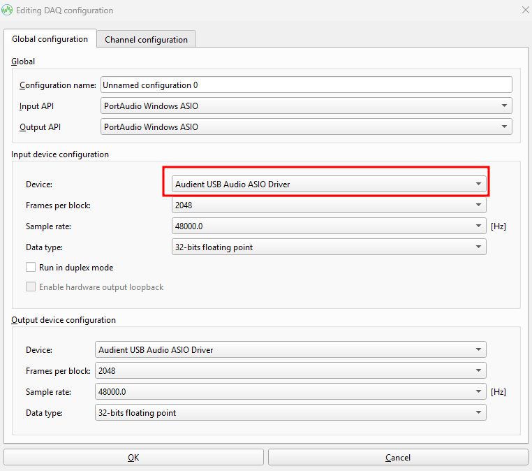
Once installed, the DAQ configuration in ACME will show the ASIO driver on API
PortAudio Windows ASIO, as shown below:
Optional: USB Driver installation for DT9837A
For interacting with the DT9837A USB data acquisition, the driver needs to be installed. A general LibUSB driver needs to be coupled to the device, which is done using Zadig.
- Go to the website, or download Zadig using this link.
- Connect your DT9837A to the PC
- Run
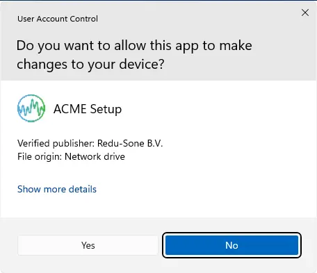
zadig-2.9.exe - For the
Zadig update policy, pressNo - When the program opens, you see the following window:
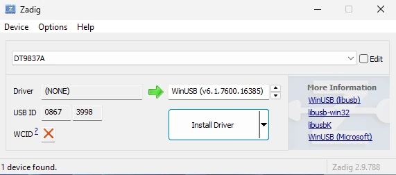
- Select the
DT9837A, if not already selected, in the drop down list - Select the
WinUSBdriver, if not already selected, in the box at the right of the green arrow. - Press
Install Driver
- Select the
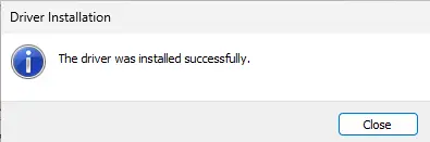
- The driver will then be installed:

- When finished you will see:
- Done! The device will now be visible in ACME's DAQ Configuration editor whenever it is connected
ACME Installation
- Double-click
acme_v<X>_installer.exe, where<X>is the version specifier:
- Click
Yes
- Click
- You will see:
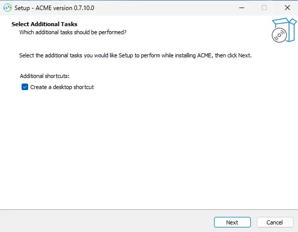
- Click
Next
- Click
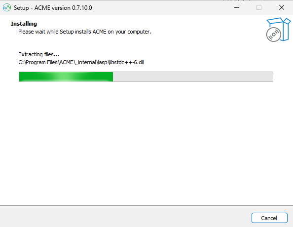
- Wait till ACME is being installed:
- When the installation is finished, the following page is shown:
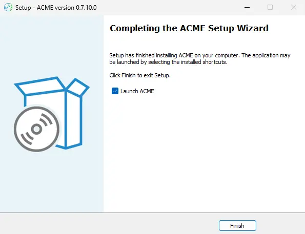
- Choose to launch ACME directly, by clicking
Finish, or choose to quit by deselecting theLaunch ACMEbox, and the clickingFinish.
- Choose to launch ACME directly, by clicking
Linux installation instructions
For installation under Linux, please make sure you have a compatible Linux version. The supported list is at System requirements section.
The commands below can be copied over using the mouse and the blue copy
button. And can subsequently be pasted in the terminal using the keyboard
shortcut <CTRL>-<SHIFT>-<V>.
After downloading the installer from the ACME download
page, run the following command in the
terminal, in the directory where the .deb file is stored:
sudo apt install ./acme_vX.Y.Z_amd64.deb
replace X.Y.Z with the appropriate version. After this, ACME will be
available in the Applications menu, and can be started as such.
note
The ./ is mandatory for apt to understand that it is a local
installation, not a package from the configured repository.
From the command line, ACME can be started by running:
/opt/acme/acme
Disable interference on audio device
On Linux, (USB) audio devices do not require additional drivers. ACME takes
control of audio devices at the ALSA layer. However, in order to take full
control of the device, other devices should not use it. Additional devices can
the most easily set to ignore the device using PulseAudio volume control.
This tool can be started with
# Run this only when the command is not yet available
sudo apt install pavucontrol
# Start pulseaudio
pavucontrol
In PulseAudio Volume Control, got to the Configuration tab, set Profile
to Off for the device that has to be controlled by ACME. Below, an example
is shown where the Audient EVO 16 is ignored by PulseAudio:
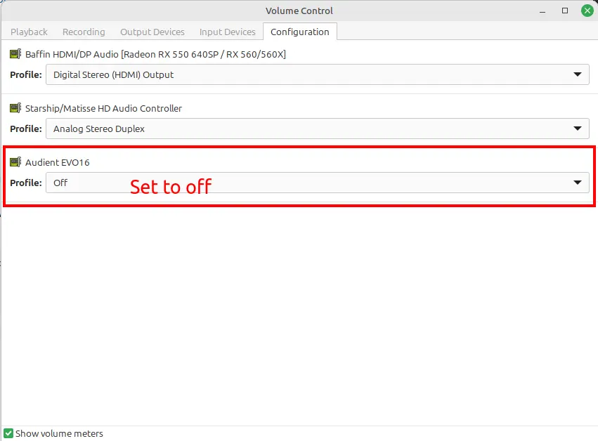
This setting is automatically stored and needs to be done only once for each device.
DT9837A configuration
ACME takes control of the DT9837A DAQ box using usb. This requires additional
permissions to be set. Please run the following commands to enable control of
the DT9837A. Open a terminal and execute the following commands:
# Download udev rules
curl https://raw.githubusercontent.com/mccdaq/uldaq/refs/heads/master/rules/50-uldaq.rules > 50-uldaq.rules
# Copy over to udev directory
sudo cp 50-uldaq.rules /etc/udev/rules.d
# Reload udev rules
sudo udevadm control --reload-rules
# Remove the local file, not necessary anymore
rm 50-uldaq.rules
Uninstalling ACME
Run the following command to remove ACME from your system:
sudo apt remove ascee-acme
License
ACME requires a valid license. After launching ACME, a dialog pops up in which the license key can be entered.
- Machine ID: Unique identifier of the computer hardware. If you need to update your hardware, please contact us. We will migrate the license to your new hardware.
- Enter / change license: Enter the license key.
- Request trial license: If you do not have a license, you can request a 30-day trial license. This trial license is activated immediately.
- OK: Click when you are finished activating the license. If no license is activated or if it has expired, ACME will shut down.
An internet connection is required to activate a license or to request a trial license. The license is tied to the computer once it is activated. Some licenses can be activated on multiple computers.

After entering a license key, the background turns green to confirm its validity.

Menu bar
The menu bar is located at the top of the screen.

It is organized as follows:
-
File
- Open measurement folder
- Recent folders
- Reload measurement folder
- Exit
-
Actions
- Toggle output stream
- Toggle input stream
- Start measurement1
- Rescan DAQ devices
- Calibrate sensor1
- Calibrate µZ system2
-
Settings
- Post processing
-
Help
- Open user guide in browser
- Show license agreement
- License key info
- Restore to default
- About
Detailed information
The items which might require more explanation are are discussed below.
Open measurement folder
All measurement files will be stored here. Any exports are saved here by default. It also contains the postprocess state, which keeps track of what figures are plotted.
Rescan DAQ devices
If a DAQ device is connected to the computer while ACME is running, it does not recognize the device. Press this button to scan and recognize the new device.
Calibrate microphone
This opens a tool to determine the sensitivity of the microphone, which is required for measuring absolute sound pressure levels.
-
The
Calibrate µZ systemaction is only available if the µZ module has been purchased. ↩
Calibrate sensor
The sensor calibration wizard helps to calibrate a sensor. This is required to measure absolute levels.
note
The calibration procedure requires a calibrator, which excites the sensor at a known level and frequency. A discrete selection of levels and frequencies is available in ACME. If your calibrator is of a different specification, please contact us and we will add support for your calibrator as soon as possible.
The sensor calibration wizard can only be opened if the input stream is running. Make sure the active input stream uses the DAQ device and sensors you want to calibrate.
The available settings in the wizard are explained below:
- Quantity: The type of sensor you are calibrating. Available options are:
- Acoustic pressure
- Acceleration
- Channel: The channel on the DAQ device to which the sensor is connected
- Frequency: Frequency of the excitation signal, generated by the calibrator
- Level: Level of the excitation signal, generated by the calibrator
- Store measurement: If this box is ticked, the calibration measurement will be saved in the current measurement folder. This can be useful for debugging purposes.
- Calibrate: Starts the calibration measurement and analysis
- Result: Displays the calculated sensitivity
- Apply: Applies the calculated sensitivity to the current DAQ configuration
- Close: Closes the sensor calibration wizard
- The wizard is closed without applying the calculated sensitivity

When using the sensor calibration wizard, keep the following things in mind:
- Before clicking the
Calibratebutton, remember to:- Let the IEPE power supply (if applicable) stabilize. This can take one minute after having started the input stream.
- Activate the calibrator
- Before applying the calculated sensitivity:
- Check whether the result is plausible. If it is off by an order of magnitude, the calibrator might have a leak, have been mounted incorrectly or be set to the incorrect level.
- After clicking
Apply:- Applying the calibration result restarts the data streams. If any of the enabled channels use IEPE, they will need to stabilize again.
- If calibrating multiple sensors in a row:
- Make sure to apply the calculated sensitivity for each microphone before calibrating the next sensor.
Toolbar
The toolbar is located near the top left of the screen and contains commonly used buttons.

Buttons
- Open measurement folder: Change the working folder in which ACME stores the measurements.
- Enable/disable the input stream: If in the DAQ configuration is set to duplex mode, this enables the duplex (input and output) stream.
- Enable/disable the output stream: No function when in duplex mode.
- Start measurement: Start a measurement with the settings defined in the Measure tab.
- FFT settings: Show the power spectra settings. For more information, see the FFT Settings page.
FFT settings
Power spectra estimations are done using Welch' method of spectral averaging. Periodograms are computed using the discrete Fourier transform, which uses the well-known Fast Fourier Transform as algorithm. We also refer to the power spectra estimation settings as the FFT settings.
The Fast Fourier Transform (FFT) settings can be selected by clicking the purple Erlenmeyer flask in the toolbar, near the top of the screen.

This menu controls two sets of settings, depending on whether it is click in the Measure or Analyze tab.
- Measure tab: Real Time Spectrum Viewer
- Analyze tab: For plotting any frequency domain measurement result
The button pops up the following dialog:

The settings are as follows:
| Description | Typical value (Measure tab) | Typical value (Analyze tab) | |
|---|---|---|---|
| FFT length | Number of samples within the FFT window. A long window yields a higher frequency resolution, at the cost of slower updates (real time viewer) and more variance. | 8192 | 48000 |
| Window type | The raw data is windowed before applying the FFT. Windowing affects the shape of spectral leakage.1 | ||
| Overlap | Overlap between successive windows. Without overlap, samples at the edge of the window are weighted less. A higher number is more accurate, at the cost of being computationally more expensive. | 0%: fast | 75%: accurate |
The resulting frequency resolution is calculated with:
In which is the sample rate and the FFT length. A sample rate of 48 kHz and an FFT lenght of 48 k result in a frequency resolution of 1 Hz.
Available windows are:
- Hann
- Hamming
- Bartlett
- Blackmann
- Rectangular
The difference between the Window types is subtle and is beyond the scope of this user guide. An exception is the Rectangular window, which turns the windowing function off and is unsuited for most analyses. The Hann window is a good all-round choice.
note
There is a special case for analyzing pure tones, when exactly an integer number of periods fits within the FFT window. In this case, a Window makes the results worse. The best result is obtained with the Rectangular window, in combination with a large FFT length.
-
See for more information: https://en.wikipedia.org/wiki/Spectral_leakage ↩
Measure tab
Access the Measure tab by clicking its tab:

The various functions are explained in the subchapters.
Configure Data AcQuisition (DAQ)
A DAQ configuration defines the device used for generating signals and reading measurement data. ACME provides an API abstraction layer around a DAQ, and is able to work with different API's to read/write signal data. The easiest way to read signal data in ACME is by using an audio interface.
Managing DAQ configurations
On the Measure tab, create a new device configuration by right clicking on
the dropdown box in DAQ configuration:
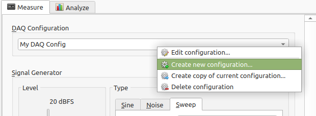
Here you can choose to:
- Edit the current configuration (if any)
- Create a new configuration
- Create a new configuration by copying the currently selected configuration
- Delete a configuration
DAQ configuration presets are stored on your computer right after creation and will be visible every time you restart ACME.
Editing a configuration
Global settings
When you edit an existing configuration, or create a new one, a dialog will open:
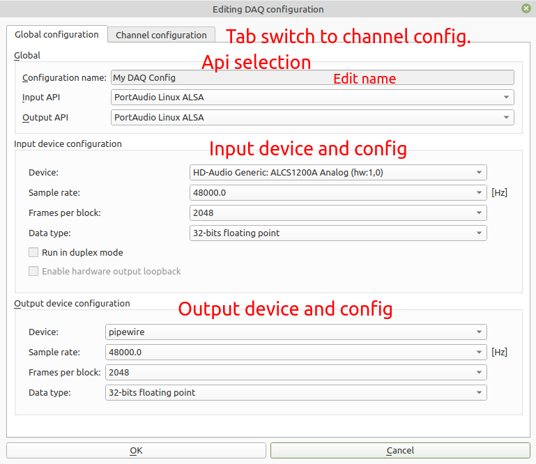
The DAQ configuration has two tabs. The first is the global configuration. The settings apply to both input and output settings. You can control input and output independently, but the configurations stores settings for both input and output simultaneously. ACME allows the usage of only one input and one output device at the same time.
- The
Configuration nameis a free text field where you can enter the name of the configuration. Duplicate names are not allowed. - The Input API / Output API show the currently selected API for the input and output.
- When a device supports duplex mode, the input and output can be coupled to
the same device. In that case, the
Outpput device configurationis greyed out, and theInput device configuration settingsapply to both input and output. - For the
Input device configurationthe sample rate can be set, this is the amount of samples that are taken per second (for each value). Lower values allow for smaller measurement file size, but also limit the highest maximum frequency that can be analyzed. - The
Frames per blocksetting is advanced, and determines the real time latency in the real time viewer. Too low values might result in buffer X-runs. Advised is to leave this value to the default of 8192. Data typeis the format for which samples obtained from the device. The allowed settings here are dependent on the device and the device driver. Floating point values are the most precise, but sometimes they are already converted from fixed point. This depends on the underlying device. It is advised to use either 32 bits fixed point of floating point.- The
Run in duplex modecheckbox switches the device to duplex mode. This lets the input and output stream run on the same pace. This is not supported by all devices. - For some devices, such as the DT9837A, a hardware loopback exists. In that case this button is enabled and an artificial input channel appears, that copies over the output signal generated with the Signal generator.
tip
If you have detailed information of the sample resolution of the used device / sound card, you can set the value of the data type accordingly. ACME stores the raw data in that sample format. For example, if the device has 16 bit resolution, the resulting measurement files will be half that of the case of 32-bits.
Channel settings
The second tab contains settings for each channel. Depending on the selected API / device combination, some settings might be grayed out.
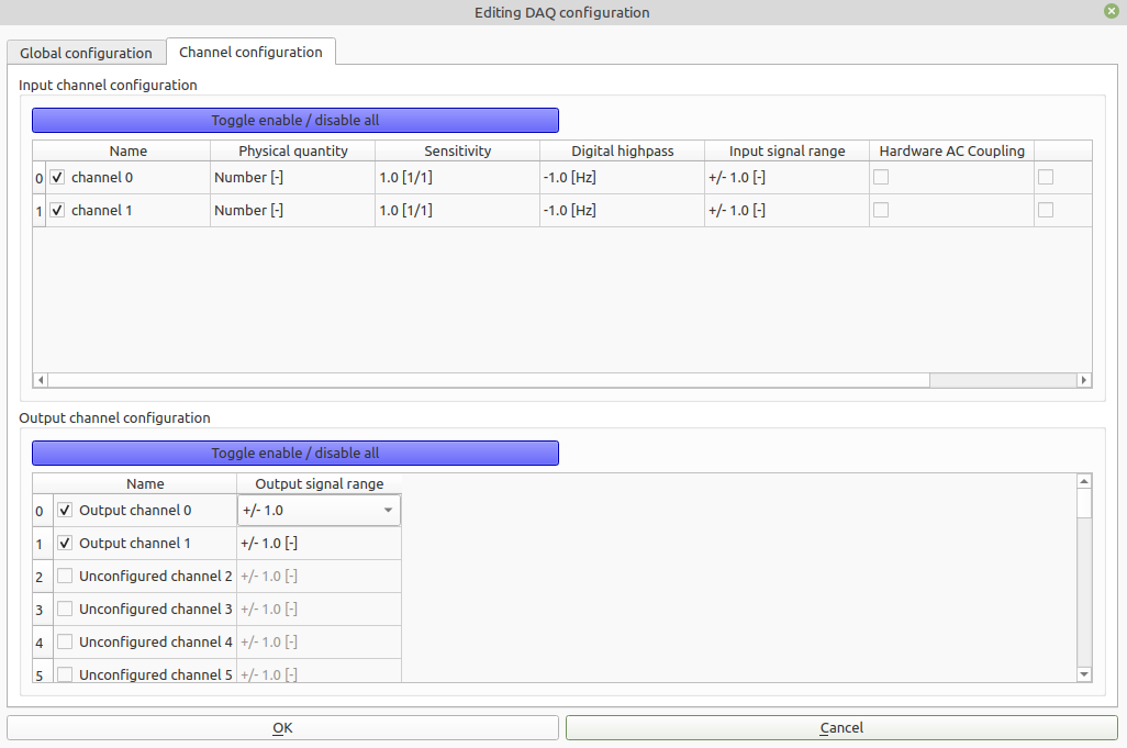
Depending on the selected input / output device, the available input and output channels is listed. From the given channels of a device, a subset can be enabled for input. These have to be checked next to the name.
- The checkbox next to the
Namefield toggles enabling this channel. Any channel not enabled is not visible in thePPM,Real time viewernor taken into account in a measurement. - The
Namefield allows for a unique name for each channel. Duplicate names are not allowed. - The
Sensitivityfield allows for setting the sensitivity. See background info below. Physical Quantityis the kind of signal that is measured ultimately and depends on the attached sensor. For a microphone, this is acoustic pressure. Changing this setting is useful e.g. for measuring sound pressure levels, and sets the proper reference levels when postprocessing.- A
Digital highpassapplies a first order digital highpass filter to the incoming data, before storing. This can be used to remove unwanted DC offset from the measured signal. When the frequency value is <=0, the digital highpass is turned off. Otherwise, it determines the cut-on frequency of the used digital highpass filter. Hardware AC couplingis another option to remove unwanted DC offset from the measured signals. If the device supports it, checking this box will enable a hardware AC coupling. This can be done, for example, by placing a capacitor in series before the ADC. The combination ofDigital highpassandHardware AC couplingis possibly, but superfluous.IEPEis a sensor power supply. This can be turned on for some sensors, for example measurement microphones and accelerometers.
warning
Turning on IEPE lets the device put a bias voltage of (> 10 V) on the channel. If your channel configuration is incorrect, it might harm the incorrectly connected device.
Sensitivity settings
The sensitivity has a unit of , where is the unit of the physical quantity and the unit of the data provided by the DAQ. For example when measuring acoustic pressure with an audio interface, the sensitivity has unit Pa. When in this example DAQ provides calibrated voltage data, the sensitivity has unit V/Pa. The following equation is applied to scale the raw data:
where is the physical measured quantity for channel and is the sensitivity for this channel. When data is stored as floating point, this equation is directly applied in this form.
Fixed point data caveats
Fixed point data is interpreted as fraction of full scale. So for fixed point data, the value is computed as
where is the maximum positive value that can be stored for the integer data. For example, for 16-bit integers this value is , for 32-bits integers this is .
When fixed point data is shown, it is always scaled to this maximum value, representing a number between -1 and 1.
Signal generator
The signal generator supplies the signal for a measurement. It consists of three parts:
- Type: Adjust the signal.
- Gain: Slider for adjusting the output level. Press
Start/Stopto enable of disable the generator. - Equalizer: Modify the spectral content.
note
The generator can only run when an output or duplex stream is running.

Type
The generator supports three types:
- Sine
- Noise
- Sweep
Sine
Generate a continuous tone with a fixed frequency.

Noise
Generate white or pink noise. Pink noise has a Color 0-dB point parameter. The
noise is only pink from this frequency up. A higher Color 0-dB point results in
a stronger power spectral density, within the pink range. The parameter
Interruption period makes the generator alternate between noise and silence.

Sweep
Generate a sweep. It has the following parameters:
- Sweep type: Sets whether the frequency increases (decreases) linearly between to start and stop frequency or exponentially. An exponential sweep puts equal power in each octave and is sometimes called a logarithmic sweep. If the results are to be viewed on a logarithmic frequency axis, use the exponential sweep.
- Sweep repetition: Sets whether the sweep increases in frequency, decreases in frequency or has an increase followed by a decrease.
- Start frequency: Sets the lower bound of the sweep.
- Stop frequency: Sets the upper bound of the sweep.
- Sweep time: Sets how fast the signal sweeps through the frequency range.
- Quiescent time: Adds a silent phase after each sweep.

Gain
The slider does not directly control the signal level. The peak output level depends on the signal type and equalizer settings. Consider the following chain:
[Type] ➔ [Gain] ➔ [Equalizer]
The raw output of Type is set to peak at 0 dBFS, for the Sine and Sweep output types. The gains of the Gain slider and Equalizer are then added. For the Noise output type, the peak value is not defined.
warning
The peak level can be higher than the setting of the Gain slider, if the Noise type is selected or if the Equalizer is enabled.
For Sine and Sweep output types, the peak level matches that of the Gain slider,
if the equalizer is disabled. A value of 0 dB then results in a full scale signal.
Equalizer
Right-click the preset box to create a new equalizer:

After entering a name, the settings window will show:

Adjust the sliders as desired. Scroll to the right to view the higher frequency bands.
Connect all levels will make all sliders move simultaneously. Reset all levels sets each band to 0 dB.
To disable the equalizer, press the Disable EQ button.
Measurement settings
The Measurement box contains the settings for the measurement.

Settings
The optional counter adds an underscore and a two digit number to the file name. It uses the lowest two digit number which has not already been taken. A third digit is added when required. This is handy when performing multiple measurements, which do not need individual annotations.
The measurement ends after Measurement time, unless Measure indefinitely is checked. Then it must be stopped manually.
The signal generator can automatically start together with a measurement, by checking Control signal generator. Because of input and output buffers, the measurement misses the first part of the generated signal. The measurement can wait for it by using a value for Measurement delay of at least two times the buffer size. In case of 8192 samples and a sample rate of 48 kHz, this equals 0.34 s.
For the Measurement type, the following options are available:
- Generic
- Insertion loss
- µZ1
The Generic option does not need additional explanation. The other options are explained in their own parts of the user guide.
Start
After clicking Start measurement, a window is shown with the measurement progress:

note
A measurement can only be started when the input stream or duplex stream is running.
tip
Measurements can also be started with the spacebar key.
Notes can be added as a Measurement comment while it is running. The measurement automatically stops after Measurement time has elapsed, unless Measure indefinitely was checked. If desired, the measurement can be stopped manually in two ways. If the result should be kept, click Stop and save. If the result should be discarded, abort by clicking the X in the top right corner.
Once the measurement is ready, it is added to the Measurement list on the Analyze tab.
-
The
µZoption is only available if the µZ module has been purchased. ↩
Signal monitor
The input signals are monitored on the signal monitor. It consists of three parts:
- PPM: Peak programme meter
- Real time signal viewer: Time domain view of one input channel
- Real time spectrum viewer: Frequency domain view of one input channel

Peak Programme Meter
The Peak Programme Meter (PPM) shows the peak level for each input channel. In one eyesight it shows the signal levels.
As the name suggests, the meter responds to the peak signal values. It can be used to help set the signal generator level or gain knobs in the system. Ideally the signal is as strong as possible, without overloading the input. A typical target level is -10 dBFS.

Features
For each channel there is a vertical bar. The bar is updated each time the DAQ sends a block of data and is green under normal circumstances. If clipping is detected, the bar turns red. To make it easier to read the peak levels, a horizontal line holds the peak value.
Options
Right-click inside the PPM to open an options menu. It has two settings:
- Minimum visible level: Sets the vertical range.
- Decay rate: Sets how quickly the bars drop, after the peak has passed. It does not affect the horizontal line that holds the peak value.
Minimum visible level

Decay rate

Real time signal viewer
This viewer shows the time domain data of one input channel.

It has two settings:
- Channel selector: Select the input channel with the drop down menu near the top. Only one channel can be viewed simultaneously.
- Time history: Adjust the slider to set the time scale.
Real time spectrum viewer
This viewer shows the spectral content of one input channel.
By default, the viewer is frozen to lessen the computational load. Click Unfreeze to enable it:

A blue line will be drawn:

Settings
- Freeze: Hold the current graph for inspection. It also stops the computational load.
- Reset: Clear the time history, related to
Time weighting. - FFT settings: See FFT settings.
- Settings menu: See below.
Settings menu
Select the input channel to be viewed and what property should be calculated. The settings shown below work for most situations. More information about the Power Spectra Settings can be found on the page Power Spectra.

Analyze tab
Access the Analyze tab by clicking its tab:

Overview
The analyze tab is divided into three sections:
- Measurement list: red
- Compute: green
- Plot area: blue

The vertical divider (purple line in the image below) between the computation settings (left) and plot area (right) is draggable. If it is dragged to far to the left some of the options may become (partially) obscured.

Workflow
To plot one or more measurements, select them from the measurement list, pick the desired computation settings and click Compute. A plot is created in the plot area. Only compatible measurements can be plotted simultaneously. In practice, this means that they must share the same DAQ Configuration.
The various sections are explained in the corresponding subchapters.
tip
If the Compute button is disabled, it likely means that the measurements you selected are not compatible. In this case, try plotting one measurement at a time.
Measurement list
The measurement is located in the top left of the Analyze tab and lists the measurements of the current measurement folder. See Toolbar how to change this folder.
- Folder: shows current measurement folder
- Select All / None: select all or no measurements
- Select new: select recently added measurements
- Filter: search measurements
- Name: click to sort by name
- Timestamp: click to sort by date and time when the measurement was performed
- Comment: click the field next to a measurement to add a comment

Hover
Details are shown when the mouse hovers over a measurement:

Right-click
Right-clicking on a measurement opens a menu. This also works if multiple measurements are selected.

Delete selected measurement(s)
Right-click --> Delete selected measurement(s) will ask for a confirmation, before deleting the measurements. Measurements can also be deleted by pressing the Del key on the keyboard.

Export selected measurement(s)
Right-click --> Export selected measurement(s) will export them as wave audio files. They are exported to the measurement folder and get the same name as the measurements.
Supported output type are:
- 32 bit float
- 16 bit integer
- 32 bit integer
Normalize maximizes the amplitude without clipping. If Overwrite existing files is checked, existing wave files with the same name will be overwritten without warning. If left unchecked, the measurements are not exported if a wave file with the same name already exists.

Edit measurement metadata
Right-click --> Export measurement metadata... opens a screen with detailed information and allows you to change the channel configuration.

Computing results
The computation settings are located at the bottom left of the Analyze tab.
They contain the following items:
- Start time: select from which point the data should be processed - will be set to the start of the signal by default.
- Stop time select up to which point the data should be processed - will be set to the end of the signal by default
- Compute: choose what to calculate
- Compute-specific settings: the contents of this sub-menu depend on what has been chosen at
Compute - Output figure: select in which figure the results should be plotted.
- Compute button: press to calculate and plot
- Auto compute: automatically compute future measurements

Start and stop position
The start and stop position select what part of the measurement is to be processed. Usually, they can be left at their default values, which uses the whole measurement. This option is disabled if multiple measurements with different lengths are selected.
Compute
This setting determines what is calculated. It offers the following options:
- Sound level meter - statistics
- Sound level meter - time dependent
- Power spectra
- Insertion loss
- µZ tool1
These options are further described in their respective sections.
Output figure
The option Output figure sets where the calculated result should be plotted. A result can be plotted in a new figure, or in any compatible existing figures. A figure is compatible if it has the same axes (with or without phase) and contains similar data, of the same quantity. For example, it is not possible to plot sound levels and a waveform in one figure.
Auto compute
If you are performing many similar measurements and want to inspect them on the go, ACME can plot them automatically. This function is enabled with the Auto button.
note
Before using the auto compute functionality, at least one measurement must be plotted manually. This selects the right settings. After that, ACME continues using the same settings.
The procedure is as follows:
- Perform a measurement
- Go to the
Analyzetab - Select the right computation settings
- Click
Compute - Enable auto compute by pressing the
Autobutton - Go the the
Measuretab - Perform other measurements
- Future measurements will automatically be plotted
If ACME is restarted or if the DAQ configuration has changed, the channel configuration could have changed. The change could make the computation settings invalid. For that reason, auto compute will be disabled. Manually plot one measurement and click the Auto button to re-enable auto compute.
-
The
µZ toolis only available if the µZ module has been purchased. ↩
Sound level meter - statistics
The sound level meter - statistics computes the sound levels within octave or third octave bands. It operates on one channel and takes the statistics across the whole measurement time. Three statistics are available:
- Peak sound level (Lpk)
- Maximum sound level (Lmax)
- Equivalent sound level (Leq)

- Channel: channel to take the statistics of
- Statistics type: Lpk, Lmax or Leq
- Time weighting for Lmax: smooth out peaks; only applies to Lmax
0.1 ms; Fast (0.125 s); slow (1 s); 10 s - Frequency weighting: A, C or Z
- Frequency bands: octave or third octave
- First band: limiting the number of bands helps to keep the figure easy to read
- Last band:
Peak sound level (Lpk)
This is the strongest sound anywhere in the measurement, without time weighting to smooth out short peaks. Even though there is no time weighting, the bandpass filters for each band still mean that there is no instantaneous reaction to a short peak, especially at the lower frequency bands.
A sine wave has an Lpk of 3 dB above Lmax or Leq.
Maximum sound level (Lmax)
This is the strongest sound anywhere in the measurement, with time weighting to smooth out short peaks.
note
The time weighting filter requires run-in time. The result is only correct if the measurement time is much longer than the time weighting.
Equivalent sound level (Leq)
This is the average power. It can be viewed as the level that a sine wave would have, to have the same average power as the measuement.
Example
An example plot with all three statistics is shown below.

Sound level meter - time dependent
The sound level meter - time dependent computes the sound levels within octave or third octave bands. It operates on one channel and plots the result as a function of time. Furthermore, it can plot the raw time domain data.
Power spectra
Power spectra computes the frequency domain data of the measurement.
Output type
The following output types are available:
- Auto power
- Bode diagram
- Signal coherence
- Transfer magnitude
- Transfer phase
They are further explained below.
Auto power
Auto power shows the average spectral content of channel Auto power channel.
It is the sum of the positive and negative frequencies, so the plot shows the
total signal power at this frequency bin. This corresponds to what a sound
level meter would do. The power is plotted on a logarithmic (dB) scale, with a
reference depending on the type of signal.
- For acoustic pressure, the reference is 20 µPa.
- For voltages, the reference is 1 V.
- For unscaled numbers, the reference is the rms level of a sine wave with unit amplitude, which is .
here are some examples / properties of these definitions:
- Assuming no spectra leakage and a rectangular window, an unscaled sine wave with an amplitude of 1.0 will have an auto power of 0 dBFS ("decibel full scale").
- An acoustic wave with an amplitude of 1 Pa rms, will show up with an overall level of 94 dB SPL.
- An acoustic sine wave with an amplitude of \sqrt{2} Pa, will show up with an overall level of 94 dB SPL.
- For white (Gaussian) noise, represented as unscaled numbers with variance of 1.0 and zero mean, up to the Nyquist frequency has an expected overall signal power of 1.0, and 0.0 above the Nyquist frequency., Therefore the expected auto power in each frequency bin . Therefore computed level in each bin is: = dBFS.
Note that due to this, for broadband signals the height of the auto powers in the spectrum depend on the frequency resolution: the higher the frequency resolution, the lower the levels. On the other hand, for narrow band signals, the height of the peaks are more / less independent on the frequency resolution.
To compute the signal auto power, select the right measurement(s) in the
Measurement List, select the Auto power channel, frequency weighting and
possible smoothing:

Ten press Compute.
Bode diagram
This type plots both the estimated magnitude and phase of a transfer function between two channels.

The transfer function is taken from Input channel to Output channel. For
best performance, set Reference channel to the channel with the lowest noise.
See 'Reference channel' below for more information.

Signal coherence
The coherence between two signals is useful to check the signal to noise ratio and linearity. A value of 1 represents perfect coherence (the signals are perfectly related) and a value of 0 represents completely uncorrelated signals. The signal coherence is defined as:
where is the cross-power spectrum estimate from channel to channel .

note
The signal coherence depends on the FFT length, as set in the FFT settings. It should not be taken as an absolute measure.
Transfer magnitude
This is the magnitude part of the Bode diagram.
Additionally, Smoothing is available.

Transfer phase
This is the phase part of the Bode diagram.

Options
- Auto power channel
- Frequency weighting
- Input channel
- Output channel
- Reference channel
- Smoothing width
Start by selecting the Output type. Depending on the choice, some items are greyed out.
| Auto power | Bode diagram | Signal coherence | Transfer magnitude | Transfer phase | |
|---|---|---|---|---|---|
| Auto power channel | ✓ | ||||
| Frequency weighting | ✓ | ||||
| Input channel | ✓ | ✓ | ✓ | ✓ | |
| Output channel | ✓ | ✓ | ✓ | ✓ | |
| Reference channel | ✓ | ✓ | ✓ | ||
| Smoothing width | ✓ | ✓ |
Auto power channel
This is the channel for which the auto power is computed.
Frequency weighting
Human hearing is less sensitive at low and high frequencies. Moreover, the frequency sensitivity depends on the level of the sound source as well. Frequency weighting can be applied as a coarse representation of that. The weightings are according to the IEC 61672:2003 standard.
- A: A-weighting
- C: C-weighting
- Z: no frequency weighting
Input channel & Output channel
Some Output types work on two channels. The types Bode diagram,
Transfer magnitude and Transfer phase describe a transfer function from
Input channel to Output channel. The output type Signal coherence also
requires two channels, but it does not matter which one is assigned to
Input channel and which to Output channel.
Reference channel
Computing a transfer function between Input channel and Output channel is
most accurate if ACME knows what channel is lowest in noise. This can be
another channel alltogether. If the signal generator is used to perform the
measurement, a low noise channel with the lowest noise is obtained by looping
back the output to another input channel. Set the Reference channel to this
loopback channel. If the signal generator is not used, then the lowest noise
channel usually is the Input channel.
Smoothing
Smoothing makes the graph easier to read, by removing details. It is only
available on output types Auto power and Transfer magnitude. As power
spectra are about the frequency domain, the data are always plotted on a
logarithmic x axis. Fractional octave smoothing has been chosen to keep the
window width visually constant.
warning
Smoothing changes the absolute levels, and thereby change the overall signal power. If smoothing is applied, the overall signal power (obtained by summing up the power in each frequency bin) is no longer accurate.
Insertion loss
Insertion loss is the reduction in sound pressure level, when a device-under-test (DUT) is added to a system.
Measure
ACME can determine the insertion loss by comparing two measurements:
- System without DUT (reference)
- System with DUT
First the reference measurement must be performed. Once this is finished, it will remain valid for 12 hours and will automatically be linked to all future measurements. Next, perform the measurement with DUT.
Reference measurement
- Select
Measurement type->Insertion loss - Tick the box
Reference measurement

Measurement with DUT
The last reference measurement is shown in the box Last reference.
- Select
Measurement type->Insertion loss - Untick the box
Reference measurement

Analyze
Insertion loss builds on Power spectra. The settings of at
Power spectra are applied to both
measurements individually, after which the results are subtracted from
eachother. The difference is plotted as the insertion loss. Any smoothing is
applied before the results are subtracted.
From Power spectra, only the output types Auto power and Bode diagram
can be used with insertion loss.
The following settings are available:
- Reference measurement: if multiple reference measurements are available, select which is to be used
- Switch sign: multiply by -1, in case the reference and DUT measurements are swapped
- Plot with phase: plot the phase as well

Example
An example is shown below. The system is a resonant tube with a loudspeaker on one end and a microphone on the other end. The DUT is a constriction, which can be placed in front of the microphone.
First, the Power spectra settings.

The resulting bode diagrams are as follows...

...and the insertion loss is the difference between them. Note that the insertion loss is positive, even though the DUT decreased the sound pressure level at the microphone.

Plot
The plot area is located on the right side of the Analyze tab.
- Tabs for each figure
- Reset axes
- Undo
- Redo
- Move
- Zoom
- Cursor position
- Change layout
- Plot operations
- Save (image)
- Preset for x axis
- Fit x axis to data
- Fit y axis to data
- Undo closing the last figure — stores up to 10 figures

Some options are not available if no figure is present.
The preset button 20 Hz ... 20 kHz is only available on a logarithmix x axis.
Legend
The legend automatically tries to find the location where it leaves a clear sight on the plotted lines. It can be manually dragged to any other position or disabled in the menu Change layout. If more than 20 lines are visible simultaneously, it is disabled.
Change layout
In this menu, the formatting of the labels and the settings of the axes and can adjusted.
The yellow arrows on the right side are 'undo' buttons.

Plot operations
The plot operations menu contains the list of plots. This menu offers the options to change the line style, apply mathematical operations, reorder the plots or export the data. Depending on the number of plots selected, some buttons can be disabled.
- Plot list
- Select & remove
- Operations
- Arrange

Plot list
This area lists all plots within the figure.
- Checkbox: a plot is selected when this checkbox is ticked; the selection is used at the buttons at
Select & remove,OperationsandArrange - Name: for your own reference
- Channel: lists
Auto power channelor (TF input,TF output) for power spectra - Line color: click the color to change
- Line width: light (1) to heavy (8)
- Line style: solid, dashed, dash-dot, dotted
- Marker: diamond, triangle etc. - not always available
- Offset: vertical offset applied to plot; to make overlapping plots visible or to move widely spaced plots together
- Visible: show / hide 10: Custom legend: tick the checkbox to modify the legend label

Select & remove
These buttons can quickly select or hide all plots, reset the line styles or remove one or more plots.
- Select All/None: select all or no plots
- Show/hide all: hide or show all plots
- Reset line styles: reset the
line color,line width,line styleandmarkerto the default cycler - Remove: delete selected plots. Plots can also be deleted by pressing the
Delkey on the keyboard.

Operations
These operations apply to the selected plots.
- Average: calculate the power average and plot the result in the same figure
- Difference: calculate the difference - y values are simply subtracted, without any conversion to power
- Sum: calculate the sum, with the option to weigh each differently and a choice between summing power or decibels
- Export: export processed data - it first opens a settings window

Export
The Export operation opens a settings popup:

- File name:
Name of the target file, without extension - File type:
File format:Comma Separated Values(.csv),Spreadsheet(.xlsx) orNumpy array(.npz) - Interpolate to logarithmic x axis:
Interpolate to 200 logarithmically spaced frequencies between 1 Hz and the Nyquist frequency. This reduces the file size and makes spreadsheets more manageable. If the option is not checked, the raw data is exported. It usually has a linear frequency axis. The frequency step size equal to the sample rate, divided by theFFT lengthat which the plot was generated. - Overwrite existing file:
Do not give a warning if the target file already exists.
When finished, click Export to export the data.
Arrange
Move the selected plots up or down in the list. Multiple plots can be moved simultaneously.

Save
Clicking the Save button opens a dialog, in which the following settings can be
entered:
- File name
- Image size

Image name
The file format is inferred from the extension of the file name. Recommended options are:
- png: good compatibility with other software
- webp: small file size (ACME uses lossless compression)
- svg: vector graphics
- eps: vector graphics
Vector graphics have the advantage that they can be scaled and still remain crisp. You can zoom in without loss of detail.
Other options might be available but are not officially supported. Formats with
lossy compression like jpg are not recommended, as their images tend to be blurry.
Image size
Various options are available for the image size. It refers to the size at which it is intended to be displayed. Both the dimensions and font size are adjusted to suit.
The option Same as on screen is different and saves the image as it is
currently shown on the screen.
| Option | Size (pixels) png | Size (inches) svg, eps | Font size (pt) |
|---|---|---|---|
| Same as on screen | as-is | pixels on screen / 100 DPI | as-is |
| Small | 800 × 600 | 8 × 6 | 16 |
| Medium | 1200 × 900 | 12 × 9 | 16 |
| Large | 1800 × 1350 | 18 × 13.5 | 20 |
µZ impedance tube

Introduction
µZ (pronounced: /'mju:zi:/) is a state-of-the-art impedance tube designed for precise acoustic testing of small material samples. The device gets it name from the symbols for micro (µ) and impedance (Z). It can be used to measure the acoustic properties of small material samples, like meshes, membranes, or vents, typically used in hearables. µZ operates effectively over a wide frequency range, depending on the specific type of device.
| System | Inner diameter | Frequency range |
|---|---|---|
| µZ-20 | 20 mm | 20 Hz - 8 kHz |
| µZ-30 | 30 mm | 20 Hz - 6 kHz |
Use cases
Although it is designed to measure acoustic properties of thin samples, µZ can also be used for regular impedance tube measurements. Combined with the ACME measurement and analysis software, the system can be used for:
- Acoustic material characterization: Characterization of the series impedance of thin materials such as meshes and membranes.
- Sound absorption measurements: Evaluation of the normal incidence sound absorption and reflection coefficient of an acoustic sample.
- Quality control: Monitoring acoustic products to ensure consistent quality.
warning
µZ is a sensitive piece of measurement equipment and its results are affected by changes in temperature. Make sure to use µZ in a well-controlled environment with consistent climate conditions.
Package contents

The µZ system is delivered in a sturdy case1 and includes the following components:
- Main tube assembly
- Contains an enclosed speaker and 4 MEMS microphones.
- Supportive base
- Calibration/measurement tube (2x2)
- Can also be used to mount samples during regular impedance tube measurements.
- Hard end cap without tip microphone (2x2)
- Used for measurements in 4 microphone mode.
- Hard end cap with tip microphone
- Used for measurements in 5 microphone mode.
- Sample holder with 0.1 cc back cavity
- Used for 5 microphone measurements on samples with relatively high series impedance.
- Sample holder with 0.5 cc back cavity
- Used for 5 microphone measurements on samples with relatively low series impedance.
- Sample holder plate
- Clamps the sample to the back cavity.
- Sample holder plate mounting tool
- Used to lock the sample holder plate in place.
- Audio interface
- Required cabling
- XLR cable (5x)
- 1/4" TRS Jack cable, short
- 1/4" TRS Jack cable, long
- USB-A to USB-C cable
- Power cable
- 5 V power supply
- Spare O-rings3
- 22.5 x 1.5 mm (5x)
- 7.0 x 1.5 mm (5x)
- 10.5 x 1.5 mm (5x)
For series impedance measurements, additional sample holder disks are required. As they are tailor-made for the samples under test, they are not part of the regular contents. We can supply them on request.
warning
µZ comes pre-assembled with the microphones already mounted on the main tube and end cap. The microphones are an integral part of the µZ system and should never be unscrewed by the user. In case the microphones have been unscrewed and remounted, proper operation can no longer be guaranteed.
-
The picture shows an old case layout. New µZ systems are delivered in cases that can fit all listed components. ↩
-
Not shown in the picture. ↩
Workflow
This overview shows the sequence of steps involved in using the µZ system. More details about each step can be found on the respective pages in this user guide.
Initial setup
These steps need to be performed once while setting up a system (consisting of the µZ hardware and a computer running the ACME software) for the first time:
-
- After installation, the sofware license needs to be activated
-
- Instructions for manual configuration of the device are also given for Linux users2
General measurement session outline
These steps need to be repeated for each measurement session:
-
Turn on the µZ hardware
-
Plug in the loudspeaker power supply
-
Plug in the Audient EVO 16
- If the EVO 16 is already plugged in but seems to be turned off, it likely is in standby mode. Wake it up by pressing the control wheel on the device. We recommend to turn off standby mode

-
-
Open measurement folder in ACME
- Create a new folder or load an existing one, to store the measurement data
-
Select a measurement configuration
- For series impedance measurements on thin acoustic samples:
- Decide whether to use the 4 or 5 microphone method and — in case of the 5 microphone method — select a cavity size
- For all other measurements: use the 4 microphone method
- For series impedance measurements on thin acoustic samples:
-
- Determine system and environmental parameters to ensure accurate measurement results
-
- Set up the hardware and software for a specific type of measurement
- In case of a series impedance measurement, a reference measurement needs to be performed before measuring the actual sample measurement
- Perform the measurement
-
- Plot various acoustic properties of the sample, as a function of frequency
- Export the plots or measurement data in several formats
-
Turn off the µZ hardware
- Unplug the loudspeaker power supply
- Unplug the Audient EVO 16
-
The Audient EVO 16 is delivered preconfigured. This section in the manual describes how to reconfigure it, should the internal memory of the device get accidentally erased. ↩
-
The software needed to store settings in the memory of the EVO 16 is not available on Linux. If you exclusively have access to Linux systems, you will need to reconfigure the EVO 16 manually every time it is rebooted, should its internal memory ever accidentally get erased. ↩
Measurement configurations
µZ can be used in two different configurations:
4 microphone mode
In this configuration only the 4 MEMS microphones that come pre-assembled along the length of the main tube are used.
note
4 microphone mode is the default method for all measurements that do not involve series impedance.

5 microphone mode
In this configuration a 5th MEMS microphone is mounted in a cavity behind the sample. This tip microphone is used to measure the sound that passes through the sample.

Each configuration has its benefits and drawbacks. The preferred configuration therefore depends on the characteristics of the samples under test. See the Selection guidelines for help on how to pick the most suitable configuration for your application.
4 microphone mode

This configuration only uses the 4 MEMS microphones that come pre-assembled along the length of the main tube. The system uses plane wave decomposition on the sound field inside the tube, to extract the incident and reflected waves (see diagram below). From this information, it can calculate the acoustic properties of the sample under test.

4 microphone mode is applicable for series impedance measurement on samples with relatively low impedance compared to the characteristic impedance of the tube. The characteristic impedance of the tube is given by1:
where is the characteristic specific acoustic impedance of air (MKS Rayl), the inner cross-section of the tube (m) and the inner diameter of the tube (m). The units of are Pas/m.
For samples with an impedance magnitude higher than 20, the plane wave decomposition method cannot accurately determine the volume velocity through the sample. As a result, the sample's acoustic properties cannot be accurately measured with the 4 microphone mode. In this case, the 5 microphone mode should be used.
-
When we specify
Rayl, we always mean MKS Rayl. 1 Rayl is 1 Pas/m. ↩
5 microphone mode

This configuration can be used to measure samples with impedances that are too high for the 4 microphone method. Since the volume velocity through these samples can't be determined by plane wave decomposition, it must be measured in a more direct way.
This is done using a 5th microphone, which is mounted in a cavity behind the sample. This microphone is referred to as the tip microphone. The pressure measured in the back cavity by the tip microphone is used to determine the volume velocity through the sample, which in turn is used to calculate the sample's acoustic properties.

The reason why this method is not suitable for measurements on very low impedance samples, is that — at low frequencies — the impedance of the back cavity becomes large relative to the impedance of the sample. This results in numerical inaccuracies.
Back cavity size
The pressure levels measured at the tip microphone are affected by the size of the back cavity. The ideal cavity size depends on the properties of the samples under test. µZ comes with cavities in two sizes:
- 0.5 cc: This is the default cavity. It works well for most types of samples. For samples with very high impedance the pressure at the tip microphone can become insufficient at high frequencies.
- 0.1 cc: In this extra small cavity, a certain level of volume flow results in higher tip microphone pressures than in the 0.5 cc cavity. This yields better measurement results at high frequencies. However, the low-frequency impedance of this cavity is higher, which can limit performance in that frequency range.
Selection guidelines
note
These selection guidelines are only relevant for series impedance measurements. For all other measurements the 4 microphone mode should be used.
Each of the configurations described in the previous sections has its benefits and drawbacks. As a result, which is the optimal configuration will depend on the properties of the sample under test and, in some cases, the frequency range of interest. The performance of the system depends on several factors, most notably the material properties of the sample, the sample dimensions and the size of the back cavity. The influence of the sample dimensions is most complex, since they affect both the impedance of the sample, and of the µZ system itself. After all, the sample holder disk is not part of the sample, but does have a hole that matches its dimensions.
Due to the complex dependencies, it is not possible to give a straightforward recommendation for which configuration to use for a certain sample size, or type of material. The user will generally have to find the best configuration for a certain sample empirically. However, some suggestions for which configuration to start with and how to select the right configuration based on collected measurement data are given below.
note
For samples with large impedance variations across the frequency spectrum, it is possible that different frequency ranges each have a different optimum configuration. But usually, one configuration will do for the whole range.
Selection procedure
The selection method consists of the following steps:
- Select an initial configuration
- Perform a series impedance measurement
- Assess the quality of the measurement results
- update the configuration choice if required
1. Select an initial configuration
The most suitable initial configuration depends on properties of the sample under test. More specifically, these are:
- Sample dimensions
- Material properties
Sample dimensions
For the sample dimensions, only count the active area of the sample, so excluding any adhesive edge. The dimension listed in the table below is the hydraulic diameter, which is defined as:
where is the cross-sectional area of the sample and is its perimeter. The hydraulic diameter of a circular sample is equal to its actual diameter. For a rectangular sample with sides and the hydraulic diameter is:
The suggested configurations for certain ranges of sample size are listed below:
| Hydraulic diameter (mm) | Suggested configuration |
|---|---|
| ≥ 5 | 4 microphone |
| 1...5 | 5 microphone (0.5 cc) |
| < 1 | 5 microphone (0.1 cc) |
Material properties
If the material properties are known, or certain properties are expected, this can be taken into account in the configuration selection. A general, qualitative guideline is listed below:
| Series impedance | Sample material properties | Suggested configuration |
|---|---|---|
| low | open, low flow resistance, compliant | 4 microphone |
| medium | 5 microphone (0.5 cc) | |
| high | closed, high flow resistance, stiff | 5 microphone (0.1 cc) |
In case of contradictory properties (i.e. a very small sample of an open material), it is recommended to give the sample size precedence over the material properties.
2. Perform a series impedance measurement
After selecting an initial configuration, perform a series impedance measurement, as described in Series impedance measurements.
3. Assess the quality of the measurement results
If using the 4 microphone method, perform the following checks:
- Plot the
Input impedance, normalized w.r.t. the characteristic impedance and check if it isn't too high.- Select the
Analyzetab in ACME and use the settings shown below. - The normalized input impedance should not exceed 20 dB. If it does, switch to the 5 microphone method with the 0.5 cc back cavity.
- Select the

- As an additional check, plot the
Series impedanceand check the results.- Use the settings as shown below.
- The normalization is arbitrary.
- Both the magnitude and phase plots should be smooth. Ragged data can indicate that the signal levels are close to the noise floor of the microphones, or that the impedance of the sample is too low to be measured. To identify the cause, try redoing the measurement with a higher signal level.
- Use the settings as shown below.

If using the 5 microphone method with the 0.5 cc back cavity, some of the data quality checks are performed automatically by ACME, while others need to be performed manually:
- If the software indicates that there is insufficient signal on the tip microphone, this indicates that the impedance of the sample is too high to be measured with this cavity size. If this error occurs, switch to the 0.1 cc back cavity.
- Plot the
Series impedance.- If the magnitude curves upwards at low (and in some cases high) frequencies, this indicates the impedance of the sample is too low to measure using this configuration. To check this, do the following:
- Plot the
Input impedance, without normalization (Absolute impedance), of the SAMPLE measurement and its associated REFERENCE measurement, in the same figure. - Click
Layoutin the toolbar below the plot window and set theY scaletoLogarithmic(see screenshot below). - If the two lines overlap or are very close together for large parts of the frequency range, the impedance of the sample is too low. Switch to the 4 microphone method.
- Plot the
- If the magnitude curves upwards at low (and in some cases high) frequencies, this indicates the impedance of the sample is too low to measure using this configuration. To check this, do the following:

If using the 5 microphone method with the 0.1 cc back cavity the quality checks are similar to those for the 0.5 cc back cavity:
- If the software indicates that there is insufficient signal on the tip microphone, check whether the output levels of the signal generator are set correctly.
- If the signal generator was set correctly, or increasing the output level doesn't help, the impedance of the sample is too high to measure with the (current) µZ system. Please contact us to discuss the possibilities to increase the measurement range of your system.
- Plot the
Series impedance, as described above for the 0.5 cc back cavity.- If the magnitude plot curves upwards at low (and in some cases high) frequencies, plot the
Input impedancesas described above for the 0.5 cc back cavity.- If the two lines overlap or are very close together for large parts of the frequency range, the impedance of the sample is too low. Switch to the 0.5 cc back cavity. If the two lines overlap over the majority of the frequency range, consider switching to the 4 microphone method.
- If the magnitude plot curves upwards at low (and in some cases high) frequencies, plot the
Examples
Below are series impedance results for 3 different mesh materials. Their properties were chosen such that one of the configurations clearly yields the best results. All meshes were measured using all three configurations. These examples serve to illustrate how the measurement results are affected, if the wrong configuration is selected for a certain sample.
Low series impedance: constant 3 M Rayl/m²
This impedance is best measured with the 4 microphone method, at least for frequencies up to 2 kHz.
Above 2 kHz, the results get quite noisy. This is due to the fact that the sample has a 2 mm diameter and is mounted on a disk with a 2 mm diameter hole. The acoustic mass of this hole results in a significant input impedance (> 20 dB) above 2 kHz, which negatively affects the quality of the measurements.
The inaccuracies of the 5 microphone method for this impedance are mainly visible at low frequencies:
- The measured magnitude of the series impedance curves upwards for both back cavity sizes, indicating that the impedance of the back cavities is high relative to the impedance of the sample.
- The measured impedance for the 0.1 cc back cavity curves up much more and over a wider frequency range than that for the 0.5 cc cavity. This makes sense, since this smaller cavity has a significantly higher impedance.

Medium series impedance: constant 80 M Rayl/m²
This impedance is best measured with the 5 microphone method using the 0.5 cc back cavity.
- The 4 microphone method yields ragged and largely inaccurate results. The impedance of the sample is too high for it too measure.
- The only range where the results are moderately accurate is between 400 Hz and 1200 Hz. However, even in this frequency range the results are not smooth.
- The 5 microphone method with the smaller 0.1 cc back cavity yields reasonably accurate results. However, the magnitude curves upwards at the low and high frequencies. Note that the deviation in magnitude at high frequencies is not accompanied by a change in phase, which indicates that it is not a physical phenomenon.

High series impedance: constant 920 M Rayl/m²
This impedance is best measured with the 5 microphone mode using the 0.1 cc back cavity.
- The 4 microphone mode yields ragged, wildly inaccurate results. The impedance of the sample is much too high for it to measure.
- The 5 microphone mode with the larger 0.5 cc back cavity yields reasonably accurate results. The main inaccuracy for this configuration can be seen at high frequencies. Here the data gets noisier, due to the signal level at the tip microphone approaching the noise floor. The volume velocity through the sample is not large enough to build up a sufficient sound pressure level within the larger back cavity.

Setup
The following sections describe the steps required to make µZ ready for use. The setup is split into three parts:
- Hardware: Setting up the impedance tube and connecting all the in- and outputs.
- Software: Creating a DAQ configuration in the ACME software that is compatible with µZ applications.
- Firmware: Configuring the Audient EVO 16 audio interface to work properly for µZ applications. This is only required if the device's internal memory is accidentally erased.
tip
For Windows users:
Windows automatically selects the EVO16 as the default soundcard. This means that all system sounds will be played through the µZ system and affect the measurements. To prevent this, you can select another soundcard as the default audio device for Windows. Alternatively, you can mute the output volume. ACME is not affected by either setting.
Hardware
This section covers the hardware setup of µZ, including cabling.
Tube

Place the main tube on the base and mount the end cap, as shown above. Remember to mount the appropriate end cap for the desired measurement configuration:
- without tip microphone for 4 microphone mode
- with tip microphone for 5 microphone mode
All part are connected using a twist and latch system. An example of the procedure for mounting a part B onto another part A is as follows:
- Position part B such that its two grooves line up with those on part A. On sample holder parts only look at the grooves that extend towards the part it's being connected to.
- Slide part B onto part A.
- Twist part B in a clockwise direction until only one of the grooves on parts A and B line up.
- Tighten the connection by closing the latches
The video below shows the procedure. Here part B is the end cap and part A is the main tube. The procedure is the same for all connecting parts.
Parts can be disconnect by following the mounting procedure in reverse.
warning
When closing and opening the latches, guide them with your fingers and prevent them from snapping with a loud click. Pinch the handle between thumb and index finger and slowly move it to its position, as shown in the video above. The snap releases enough energy to damage the surface finish of the aluminum parts. Furthermore, it sends a mechanical shock through the microphones, which can cause a change in their response. Repetitive snaps might cause permanent damage.
The main tube, calibration tube and sample holders contain O-rings to ensure airtight seals between the parts when the system is assembled. It is possible that repeatedly removing and mounting parts can cause the O-rings to fall out of their grooves. When doing measurements, periodically check whether the O-rings are still in place, especially when the results are not as expected. Spare O-rings are included with the system to replace ones that might get lost during use. If additional parts are needed, please contact us.
Cabling
Audient EVO 16
warning
The Audient EVO 16 audio interface is configured to apply power to the microphone inputs immediately on start-up. It is recommended to connect all the cables before turning on the EVO 16.
µZ comes with an Audient EVO 16 audio interface. The device can be turned on by connecting it to power using the power cable. Connect it to the computer running ACME via the USB-C cable. Depending on your operating system, additional drivers might be required to fully use the EVO 16's capabilities. For more information, check the Audio driver requirements section.
All cables are connected on the rear panel of the EVO 16. An overview of which cables are connected to which ports is shown in the picture below. Each connection will be discussed in more detail in the following.

note
The Audient EVO 16 audio interface has 8 line outputs. However, it is important that only line output channels 1 and 2 are used.
Loopback
µZ measurements require a loopback of the speaker signal. To create this loopback, connect line output 2 to mic/line input 8 using the short TRS jack cable. See picture below:

Microphones
Connect the microphones to mic/line inputs 3 to 7 on the back panel of the EVO 16, using the XLR to XLR cables. The connections are listed in the table below. The microphone indices are marked on the µZ main tube and end cap with microphone.
| Microphone | EVO 16 channel | Remarks |
|---|---|---|
| 0 | 3 | |
| 1 | 4 | |
| 2 | 5 | |
| 3 | 6 | |
| T(ip microphone) | 7 | Optional |
The channel connections are shown in the picture below. The colors indicate the channel / microphone connections. The picture shows the system in 4 microphone mode. Therefore, the tip microphone (which would be connected to input channel 7 on the EVO 16) is not shown.

The microphones will receive power from the phantom power on the EVO 16. If the EVO 16 is configured correctly, the green LEDs in the microphones will light up once the EVO 16 is plugged in, as shown in the picture below. If they don't, the EVO 16 will likely have to be reconfigured

Speaker
Connect the speaker amplifier to power using the 5V AC adapter. Once the power is connected, the LED next to the barrel connector should light up.
If using an alternative adapter, make sure to use one with the following output specifications:
| Voltage | Max. Current | Connector dimensions | Connector polarity |
|---|---|---|---|
| 5 VDC | 2 A | 2.1 x 5.5 mm | Center positive |
Connect the signal input socket of the speaker to the to line output 1 on the EVO 16 using the long TRS jack cable, as shown in the picture below.

DAQ configuration
To work with µZ, a compatible DAQ configuration must first be created in ACME.
Start ACME and open the Measure tab. Right-click the drop-down menu labeled DAQ Configuration and click Create new configuration....

This will open a dialog. In the Global configuration tab, set the settings as shown below, taking note of the following:
- The
configuration namecan be set to whatever you prefer, but it is recommended to make it something clearly linked to µZ. - The Output settings are not used, since the EVO 16 will be used in
duplex mode. Therefore, their values do not matter. - The
Input APIis operating system dependent. It should be set to thePortAudioversion for your operating system. - The exact device name for the Audient EVO 16 may differ on your system, but it will be clearly recognizable as the Audient EVO 16.

In the Channel configuration tab set the settings as shown below, taking note of the following:
- The indices of the in- and output channels in the DAQ configuration do not match the channel indices on the Audient EVO 16, since the former starts counting at 0, while the latter starts at 1. Therefore, DAQ configuration channel 0 corresponds to channel 1 on the EVO 16.
- The input channel names must be exactly as shown below, because they will be used by the µZ toolbox to determine the system configuration.
- The
tip microphonechannel should be enabled or disabled, depending on the desired measurement configuration.- If it is enabled, the software assumes that the system is in 5 microphone mode.
- Otherwise, it will assume the system is in 4 microphone mode.
- For the input channels with a microphone (not the 'spk loopback'), set:
Physical quantity:Acoustic pressure [Pa]Sensitivity: 6.700e-03 [1/Pa] 1
- In the
Output channel configurationchannels 0 and 1 must be enabled. Their names are optional, but are added for clarity.

tip
The DAQ configurations for 4 and 5 microphones can be created in one go.
First create a DAQ configuration with 5 microphones and call it 'muz 5 microphone'.
Make a copy of it by right-clicking the DAQ configuration selection box and selecting Create copy of current configuration.... In the editing dialog, untick the checkbox of the tip microphone channel. Rename the configuration to 'muz 4 microphone' and save it by clicking OK. Now you have DAQ configurations ready for all µZ use cases.
-
The input gain on the EVO16 used to be set to 0 dB for all microphone channels. In that case, the PPM should peak at -15 dB. In October 2025, we have updated the gain to +7 dB to make the PPM reflect the input range of the microphone. Now the PPM reads levels which are 7 dB higher. See the Audient EVO 16 page for instructions on how to update the gain. ↩
Audient EVO 16 configuration
Each µZ system is delivered with a preconfigured Audient EVO 16. More specifically, it is preprogrammed with the following settings:
- Phantom power is applied to mic/line inputs 3-7
- The volume control is disabled on line outputs 1 and 2, fixing them at maximum volume
- Standby mode is turned off (for units delivered after September 2025)
Should the settings be lost for some reason, they can be reprogrammed as decribed below. We recommend to configure the EVO 16 from a pc. If that is not an option, it can also be configured using the buttons on the device.
Configure from a pc
This is the recommended way of configuring the EVO 16, as it only has to be done once (unless the device forgets its settings again). This option is only available for Windows. If you exclusively have access to Linux systems, the EVO can only be configured using the buttons on the device itself.
Download software
To configure the EVO 16 for standalone operation, you will need the EVO mixer. If you are using µZ on a Windows or macOS system, it should already be installed if you have installed the device driver. If not, or if you are configuring the EVO 16 on a different computer, download and install the driver from the Audient website. Make sure to enable all options during installation.
Select settings
Once the EVO mixer is installed, you can configure the EVO 16 for standalone operation using the following steps:
-
Connect your EVO device to the computer and turn it on
-
Open the EVO mixer
-
Open the
Viewmenu from the toolbar and make sure the following options are checked:Show Analogue InputsShow Mic Pre Controls

-
For channels Mic 3 ... Mic 7:
- Turn on phantom power:
- Click the
48Vbutton to enable phantom power - Do not enable the 48V phantom power on channels Mic 1, Mic 2 or Mic 8
- Click the
- Set the gain to +7 dB:
- Click the gain knob
- The knob has no scale in the software, which makes setting it a little difficult. It has a range of -8 ... + 50 dB and each key press changes it by 1 dB.
- On a keyboard: use the arrow key
Downto move the knob to its lowest setting. - On a keyboard: press the arrow key
Up15 times, to set the knob to +7. - Check the actual value on the EVO device by pressing the button with the channel number. The display will show the current gain setting for that channel.

- Turn on phantom power:
-
Open the
Viewmenu from the toolbar and clickShow System Panel
-
In the
Routingsection of theSystem panel, open theAnalogue outputstab and set the routing forStereo 1+2toDAW Thru
-
Click
OKin the warning dialog that pops up -
Open the
Setupmenu from the toolbar and clickStore Standalone State
Your Audient EVO 16 is now configured for µZ aplications.
Configure on the EVO 16 itself
note
This method is not recommended. If configured this way, the settings are lost when the device is turned off.
The EVO 16 can also be configured through the physical buttons on the device. If it is configured this way, all settings are lost when the device is turned off. Therefore, the manual configuration procedure needs to be performed each time the device is turned on and is not recommended. However, if you do not have access to a Windows or macOS system to configure the EVO 16, this is the only option.
To configure the EVO 16 manually, perform the following actions on the front panel of the device:
-
Set the volume of the line outputs to 100 by pressing the Speaker button and turning the Control wheel.

-
For microphone channels 3 ... 7, set the gain to +7 dB and turn on the phantom power. Perform the following actions for each channel:
- Select the channel by pressing the associated number button on the front panel
- Rotate the dial clockwise, until the diplay shows "+7 Gain"
- Turn on the phantom power by pressing the
48Vbutton. The button will light up and the display will indicate that phantom power has been enabled

If the phantom power is enabled correctly and the power supply is working, the green LED in the connected microphone will light up (see picture below)

warning
Do not turn on phantom power on input channel 8, which is used for the loopback.
Turning off standby mode
The Audient EVO 16 enters standby mode to save power, if no stream is running for 5 minutes. This functionality can be turned off through
the Settings menu on the device itself.
note
This options is only available on firmware version 1.3.0 and higher. If you do not see the options listed below in the menu, the firmware version on your EVO 16 is too old.
-
Hold the Control wheel on the front panel of the EVO 16 until the
Settingsmenu is displayed
-
Turn the Control wheel until the
Sleep timeoutoption is highlighted and click the wheel to select -
Turn the Control wheel until the
Offoption is highlighted and click the wheel to select
The EVO 16 is now configured to never go into standby mode. This setting is retained when the device is turned off.
Calibration
In order to achieve accurate measurement results, µZ needs to know certain parameters about itself and the environment it's being used in. To determine these parameters, the response of the system needs to be measured in two configurations:
- Short: End cap mounted directly onto the main tube.
- Long: Calibration tube mounted between the main tube and end cap.
Since µZ is sensitive to temperature, the calibration procedure needs to be performed at the start of every measurement session. If the temperature changes by more than 2 °C (3.6 °F) over the session, a new calibration is required. ACME has a built-in reminder that discards calibrations older than 12 hours, but cannot check for temperature changes.
Procedure
To calibrate your µZ system, open the Actions menu in ACME's menu bar and
click Calibrate µZ system:

This will open the µZ calibration wizard, which will guide you through the
entire calibration process. Some additional information about the calibration
process is listed below. This information can also be found in the calibration
wizard.
Number of microphones
The calibration can be performed:
- without tip microphone: 4 microphones in total
- with tip microphone: 5 microphones in total
To include the tip microphone in the calibration procedure, enable it in the DAQ configuration. Check the compatibility chart below to see what method to use. It depends on the desired measurement configuration.
| Measurement configuration 4 mic | Measurement configuration 5 mic | |
|---|---|---|
| Calibration 4 mic | ✅ | ❌ |
| Calibration 5 mic | ✅ | ✅ |
Calibrating with tip microphone is always right. Calibrating with without tip microphone can be useful when less cable clutter is desired.
tip
Always include the tip microphone in the calibration.
Setting speaker output level
To get the best results, the speaker output should be as high as possible, without overloading the microphones. To make sure your output levels are correct, click the Check levels button in the Short calibration measurement screen of the µZ calibration wizard.

During the signals check, the speaker will play a fast sweep signal. The PPM bars should peak at around -8 dB1. A speaker output level of -44 dBFS (µZ-20) or -38 dBFS (µZ-30) usually works well.
tip
Remember the level you set in the calibration wizard. This level can be used for future calibrations and is a good starting point for µZ measurements, once the system has been calibrated.
Two-stage measurements
The calibration measurements are performed using a sweep signal. To maximize the signal quality for each measurement, an amplitude envelope is applied. For this reason, two measurements are performed for each configuration. The initial measurement is used only to calculate the amplitude envelope.
Signal checks
The µZ toolbox performs a number of checks on each measurement to determine whether the system is operating as expected. The checks include:
- Signal levels on the input channels: Are the power supplies of the speaker and all microphones enabled?
- Channel names: Is the data as expected based on the channel name?
- System identification: Is the system that's being calibrated a µZ-20 or µZ-30?
- System configuration check: Is the data compatible with a short or long calibration measurement?
If any of these checks fail, the calibration wizard will show an error message and give instructions on how the issue can be resolved.
note
If the calibration wizard shows an error of which you are sure it is incorrect (for example, a mislabeled input channel, while you are certain the channel names are correct) check all your connections and settings and restart the calibration wizard. Also check the signal generator level: If the level is too strong, the microphones may be driven into clipping. If the level is too low, the signal-to-noise ratio is insufficient for the internal checks. If the problem persists, please contact us.
Saving measurements
When the calibration wizard is closed after a successful calibration procedure, there is no need to save the measurements. Therefore this option is not offered.
Should anything happen to have gone wrong, you will have the option to save the measurements that were performed so far. These can aid with troubleshooting. If available, the definitive measurements are the most valuable to save: if one exists, it means that there were no problems with the corresponding initial measurement. Furthermore, the definitive measurements are what the calibration calculation is based on.
Troubleshooting
If the calibration wizard failed and you do not know why, save the measurements performed so far. Then plot and inspect the following items:
-
Plot the auto power spectrum of the individual channels.
- Check that all channels receive a clean signal.
-
Plot the bode diagram with the following settings:
- Input channel: mic3
- Output channel: mic0
- Reference channel: mic3
- Check that the phase is within -3°...3° over the frequency range 20...100 Hz. If not, the system has a leak. See the figure below.

-
Plot the waveform of channel: mic0.
-
Zoom out to see the whole measurement.
- Check that the signals are not contaminated by external sounds. Those could be from an impact or a Windows sound. The amplitude envelope should be mostly constant on the definitive measurement, except for several dips. Furthermore, it should be horizontally symmetric. If the envelope has a spike, which is either clearly stronger than the remainder of the envelope or makes the measurement asymmetric, that is an indication of an external sound. The figure below shows an example, with an impact at the 5 seconds mark.

-
Zoom in on one wave. The figure below shows how it should look.
- Check that the signal peaks are not clipped: the wave should look like a sine wave and not have a flattened top or bottom.
- Check that the signal is not buried in the noise floor: the graph should be smooth and not scribly.

-
-
The input gain on the EVO16 used to be set to 0 dB for all microphone channels. In that case, the PPM should peak at -15 dB. In October 2025, we have updated the gain to +7 dB to make the PPM reflect the input range of the microphone. Now the PPM reads levels which are 7 dB higher. See the Audient EVO 16 page for instructions on how to update the gain. ↩
Performing a measurement
Two types of µZ measurements can be performed:
- Series impedance measurements:
Characterize samples of thin acoustic material. - Generic impedance tube measurements:
All other measurements, e.g. to determine the sound absorption coefficient of a material.
The difference between these types is that a series impedance measurement requires a reference measurement. A reference measurement is similar to the sample measurement measurement, including sample holder and disk, except that no sample is mounted. ACME uses the reference measurement to cancel out the acoustic effects of the sample holder and disk and extract the acoustic properties of the sample itself.
Before doing any µZ measurement, keep the following things in mind:
- All µZ measurements require a valid calibration, which must be performed before the actual measurements and must not be older than 12 hours.
- The calibration must at least include all microphones that are used in the measurement.
- The calibration must have been performed with the same DAQ configuration as the one that is currently active for the measurements. If this is not the case, ACME will flag the calibration as incompatible.
Setting up the software
To perform a measurement, open the Measure tab in ACME. Everything related to setting up and performing measurements can be found here.
The following section contains information about the signal generator and other measurement settings that are applicable to all µZ measurements. Information about settings that are specific to a certain type of measurement can be found in the relevant sections of this user guide.
warning
Some of the settings discussed below are critical. This will be indicated. The system might not achieve its optimal accuracy or might not work altogether, if a different value is used.

Signal generator
The signal generator settings are indicated in the screenshot above with a black rectangle. µZ measurements can be performed using either a sweep or a noise signal. The recommended settings for both signal types are described below.
note
Sweep is often the best method for µz, because it allows for a two-stage measurement. This yields a better signal-to-noise ratio. See Two-stage measurement below for details.
important
After each measurement, the software checks the channel labeling. This check relies on a sufficiently high signal-to-noise ratio. If the software indicates that the channel labels are wrong, try increasing the Measurement time to at least 20 s.
Sweep
The recommended signal generator settings for a sweep signal are shown below. More details about the meaning of each of the settings can be found at Signal generator: Sweep. The settings shown are for a µZ-20 system1.

- Start frequency: This setting determines the lower limit of the measurement range. Data below this frequency will not be reliable during analysis. For optimum accuracy, set it to 1 octave below (factor 0.5) the lowest frequency in the desired analysis range.2
- Stop frequency: This setting determines the upper limit of the measurement range. Data above this frequency will not be reliable during analysis. For optimum accuracy, set it to ⅓ octave above (factor 1.25) the highest frequency in the desired analysis range.2
- Sweep time: This setting, together with the
Number of sweepsin the other measurement settings, determines the length of the measurement. Lowering the sweep time will shorten the measurement time, but will also reduce the quality of the measurement data. The absolute minimum value for this setting is 10 seconds. Below this value, the automatic equalization will fail. - Other settings: The other settings should be set as shown in the image above.
Noise
The recommended signal generator settings for a noise signal are shown below.

- Color 0-dB point: This changes the signal level balance between high and low frequencies. A lower value will improve the signal-to-noise ratio at the lower end of the measurement range, while a higher value results in a stronger and cleaner signal above the
Color 0-dB point. If a bandpass filter is used, there is no advantage to picking a high value and it can be left at 20 Hz. Otherwise, a sensible range for this parameter is 10 ... 200 Hz. - Other settings: The other settings should be set as shown in the image above.
Band-pass equalizer (Noise signal only)
A noise generator generates a broadband signal, containing all frequencies up to the Nyquist frequency. This excites the system at frequencies which are not of interest, as the measurement range of a µZ systems is narrower. Additionally, some samples may exhibit non-linear behavior or be sensitive to overload in certain frequency ranges and should not be excited at those frequencies.
For this reason it is recommended to band-pass the speaker signal to either the measurement range of your µZ system, or the sample under test, whichever is narrower. There is no need to expand the frequency range slightly, as is necessary for the sweep signal. In ACME, this can be achieved by applying an Equalizer to the output signal. To create an equalizer, right-click the drop-down menu labeled Select Preset and click Create new equalizer.... This will open a dialog.

In the dialog, drag the sliders corresponding to the third-octave bands that are outside the desired measurement range fully down. Leave the other sliders unchanged. The EQ shown below is set up to use the entire measurement range of the µZ-20 (20 Hz - 8 kHz).

Save and close the new equalizer by clicking OK. Then enable the equalizer by clicking the Enable EQ button.
Signal level

The optimal signal level takes the following factors into account:
- Maximize the signal-to-noise ratio
- Avoid overloading the microphones
- Avoid overloading the sample
- Avoid creating turbulence through the empty sample disk during the reference measurement3
When using a sweep. the speaker output level as used in the calibration wizard is often a good starting point for measurements with the 5 microphone method.
For other settings or configurations, the following procedure can be used to find the right signal level:
Quick check:
- Set up the system hardware as is will be used during the measurement, including the sample holder, empty disk and/or end cap. Leave out the parts out that will not be part of the measurement.
- Enable the signal generator by clicking the
Startbutton. See the image above. - Set the level slider such that the microphone channel with the highest level peaks at around -8 dB.4 5
tip
If a sweep signal is used, the Sweep time can be shortened to 2 seconds during
the test. Remember to return the parameter to its original setting before
starting the actual measurement.
Full check:
- Perform the quick check.
- In the Toolbar, open the
FFT settingsmenu. Use the following settings:FFT length: 8000Window type:Rectangular
- Set the signal generator to a
Sinewave with a frequency of 96 Hz6. - In the
Real Time Spectrum Viewer, open theSettingsmenu. Select the following settings:Output type:Auto powerTime weighting:Fast (0.125 s)Auto power channel: tip microphone (5 microphone method) or microphone 0 (4 microphone method)Frequency weighting:Z-weighting (unweighted)
- Unfreeze the
Real Time Spectrum Viewer. The graph shows a peak at 96 Hz and at multiples of it.- 96 Hz is the fundamental frequency.
- The multiples are harmonics and indicate harmonic distortion.
- If required, decrease the level slider until the level of each of the harmonics is at least 50 dB lower than that of the fundamental.
Other measurement settings
The general measurement settings can be found on the bottom half of the Measure tab in ACME. The The recommended settings for µZ measurements are shown below.

- File name: The base file name and whether to add a counter can be chosen freely by the user.
- Number of sweeps (sweep signal only): This affects the measurement time. It is recommended to use a single long/slow sweep, rather than multiple short/fast ones.
- Measurement time (noise signal only): For noise signals the measurement time can be set explicitly. The measurement quality increases with measurement time. This value should not be set below 10 second.
- Measurement type: To set up a µZ measurement, this has to be set to µZ. The options at the bottom depend on the
µZ measurement typeand will be discussed in the associated sections of this user guide. - Reference plane offset: The reference plane is the location at which the analysis will be performed. By default, it is the plane at the open end of the main tube. A positive offset shifts the plane away from the loudspeaker. A circular tube with the same inner diameter as the µZ system is assumed to be connected between the sample and µZ system. For Series impedance measurements, the offset is 0. For generic impedance tube measurements, see the explanation on the page Generic impedance tube measurements - Measurement settings.
- Other settings: The other settings should be set as shown in the image above.
Start the data streams
Before starting a measurement, first start the input and output streams in ACME by clicking the microphone button in the toolbar, as shown in the image below. This will start both streams, since the Audient EVO 16 is set to run in duplex mode.

Two-stage measurement
µZ measurements with a sweep signal are performed in two stages, just like during the calibration. An additional dialog shows the progress.
warning
Since these two-stage measurements will be equalized automatically, make sure no other equalizer is enabled when starting the measurement.
A sub-set of the checks that are performed during the calibration will also be performed here. The definitive measurement is saved automatically.
-
The frequency limits for the
Start frequencyandStop frequencyare linked to the frequency range of your µZ system. ↩ -
The quality of the measurement data is reduced near the edges of the frequency range. To ensure clean data across the entire frequency range of interest, the frequency range for the measurement must be extended. Note that analysis with the µZ tool will only return data within the frequency range of your µZ system, regardless of the specified measurement range. ↩ ↩2
-
This seldom is a problem. It can occur when using the 4 microphone method to measure an empty sample disk with a small hole, e.g. 2 mm. The 4 microphone method is generally not the right choice for those disks. ↩
-
The input gain on the EVO16 used to be set to 0 dB for all microphone channels. In that case, the PPM should peak at -15 dB. In October 2025, we have updated the gain to +7 dB to make the PPM reflect the input range of the microphone. Now the PPM reads levels which are 7 dB higher. See the Audient EVO 16 page for instructions on how to update the gain. ↩
-
Capacitative / compliant materials, like membranes, may resonate in the measurement range. If this is case, it is possible that the previously suggested signal levels will yield distorted results. If this occurs, try redoing the measurement with a lower signal level. ↩
-
96 Hz may seem to be an arbitrary choice, but it is not. For
RectangularFFT windows it is important that an exact integer number of periods fits inside the window, to prevent spectral leakage. It is also possible to set the FFT length to48000and use any integer frequency, but this makes the computation much heavier. ↩
Series impedance measurements
This section describes the required hardware, software settings and measurement procedure to determine the series impedance of a thin acoustic sample, as a function of frequency. The sample has to be thin, as it is considered a lumped element. A thickness up to 1 mm is acceptable.
Reference measurement
For a series impedance, in addition to the measurement with sample measurement, a reference measurement is required. Both measurements share the same procedure and settings. The only differences are:
- Which sample disk (empty or with sample) is mounted in the sample holder.
- Whether the checkbox
Reference measurementis ticked in ACME:

The reference measurement must always be performed before the measurement with sample. A reference measurement remains valid for 12 hours and will automatically be tied to the sample measurement.
Hardware
In addition to the main tube assembly, the following hardware is required to perform a series impedance measurement:
- Sample holder / back cavity:
- Two options: 0.1 cc or 0.5 cc. In 4 microphone mode, always use the 0.5 cc cavity. In 5 microphone mode, see Measurement configurations for selection guidelines.
- Sample holder disk (empty):
- This disk will be used for the reference measurement. Make sure that this disk has the same hole shape and size as the one with the sample on it.
- Sample holder disk (with sample):
- The hole diameter and shape in the disk should match the active area of the sample under test.
- Sample holder plate:
- This plate will hold the sample holder disks in place during the measurements and is required for an airtight seal.
- Sample holder plate mounting tool:
- Is used to lock the sample holder plate in place.
- Hard end cap with tip microphone (optional, not shown):
- This end cap should only be used for measurements in 5 microphone mode. For measurements in 4 microphone mode, no end cap should be used.

Mounting a sample
The procedure for mounting a sample in the sample holder is shown in the video below:
- Carefully place the sample on the sample holder disk, for example using a scalpel.
- Make sure the active area fully overlaps with the hole in the disk
- Press down on the sample to make sure the adhesive on the sample fully bonds to the disk and forms a seal
- With capacitative / compliant samples, be careful not to apply too much force. Doing so will strectch the sample, changing its acoustic properties
- (In case of capacitative / compliant samples) leave the sample to rest overnight
- For these types of materials the tension in the sample and thus its acoustic properties will change in the first few hours after mounting it on the disk.
- Place the sample holder disk in the sample holder, with the sample side up
- Place the sample holder plate on top of the disk
- Press down on the plate using the mounting tool and rotate clockwise until it locks
- If the plate does not fall out when holding the sample holder upside down, it is mounted correctly.
Mount the sample holder directly onto the main tube as shown in the video below. Remember to remove the calibration tube if you have just finished calibrating.
warning
The sample holders do not fit onto the calibration tube, only onto the main tube. Trying to mount a sample holder onto the calibration tube by force can cause damage to the system.
For measurements in 5 microphone mode, mount the end cap with microphone onto the sample holder. For 4 microphone mode measurements, leave the back of the sample holder open.
Sample holder disks
The sample holder disks, which are shown on the image above, are tailor-made for the samples under test. Their dimensions are as follows:
- Diameter: 17.8 mm (+0.1, -0.3 mm)
- Thickness: 1.1 mm (+0.05, -0.15 mm)
- Center hole diameter: matching the active area of the sample
There are two options for the material:
- Re-usable stainless steel
Suitable for all samples. Be careful to not scratch the surface when removing an old sample. - Disposable plastic
Suitable for meshes, but not for membranes. They can be 3D printed with a resin printer. It works best if the disk is standing on its edge. Place supports on the edge only and sand their residues off with 2000 grit paper. The center hole should be reamed to size before the final UV hardening stage.
The sample holder disk is under a bending moment when it is mounted. The resulting strain is small and does not significantly affect the back cavity volume. Even so, the strain is enough to have a measurable effect on the compliance, for some membrane samples. Therefore membranes should always be measured on a steel sample holder disk. This phenomenon does not apply to meshes, which typically are not sensitive to mechanical stress.
Software
These settings are specific to series impedance measurements. Other settings, like those for the signal generator can be found here.
Signal generator
Set up the signal generator according to Performing a measurement - Signal generator.
Measurement settings
The recommended measurement settings, for series impedance measurements on a µZ system, are shown below.

The following settings are specific to series impedance measurements and are of interest to the user. All other settings should generally be set as shown above and are explained in Measurement settings.
- µZ measurement type: Indicates how the measurement should be processed during analysis. Set to
Series impedance (4 microphones)orSeries impedance (5 microphones)depending on the hardware configuration being used. - Reference measurement: Check this box when performing the reference measurement.
- Cavity size (5 microphone mode only): Indicates what size back cavity was used during the measurement (
0.1 ccor0.5 cc). - Sample size: Indicates the active diameter or area of the sample under test. This is used to calculate the specific impedance of the sample. It must be the same for the sample measurement itself and the accompanying reference measurement.
Performing the reference measurement
- Mount the empty sample disk in the sample holder and attach it to the tube.
- Check the box
Reference measurement. - Start the measurement.
Performing the sample measurement
- Replace the empty sample disk by one with a sample.
- Ensure the checkbox
Reference measurementis unchecked. Leave all other settings as they are. - Start the measurement.
Generic impedance tube measurements
Generic measurements are all measurements other than series impedance. The measurements generally involve placing acoustic samples of non-negligible thickness inside the measurement tube. An example is measuring the absorption coefficient of a fibrous absorber.
note
The µZ system uses normal sound incidence. This is different from the ISO 354:2003 standard 'Acoustics — Measurement of sound absorption in a reverberation room', which uses random incidence.
Hardware
In addition to the main tube assembly, the following hardware is required:
- End cap, without tip microphone
- Measurements tube: This tube is identical to the calibration tube and can be used interchangeably. If two tubes are available, we recommend to dedicate one to calibration, to guarantee it remains clean on the inside.
- Sample

Place the acoustic sample inside the measurement tube. If its thickness is smaller than the tube length, it should touch the end cap and leave empty space on the other end. The sample should cover the whole cross-section of the tube, without leaving a gap to the tube wall.
Mount the end cap to the measurement tube and mount the assembly onto the main tube.
Software
These settings are specific to generic impedance tube measurements. Other settings, like those for the signal generator can be found here.
Signal generator
Set up the signal generator according to Performing a measurement - Signal generator.
Measurement settings
The recommended measurement settings for generic measurements on a µZ system are shown below.

The following settings are specific to generic impedance measurements and are of interest to the user. All other settings should generally be set as shown above and are explained in Measurement settings.
- µZ measurement type: Indicates how the measurement should be processed during analysis. Set to
Generic. - Reference plane offset: If the front plane of the sample is not located directly at the open end of the main tube, enter the offset here. Generally, samples are placed in the measurement flush against the end cap. In this case, calculate the reference plane offset by subtracting the thickness of the acoustic sample from the length of the measurement tube, which is 200 mm1. See the image below.

Performing the sample measurement
- Start the measurement.
-
For example, the reference plane offset for a 130 mm thick acoustic sample would be 70 mm. ↩
Analysis
After the measurements have been performed, it is time to analyze them. Move to the Analyze tab in ACME.

FFT settings
µZ requires specific FFT settings:
- FFT length: corresponding to 1 second; e.g. 48000 if the sample rate is 48 kHz
- Window:
Hann - Overlap: 75%
To prevent errors, ACME overrides the settings that are manually entered in the settings dialog. It only does so for µZ measurements.

Compute settings
µZ tool
Select the µZ tool.

The other tools like Sound Level Meter - time dependent and Power Spectra work on the measurements as well, but access the raw microphone data instead. They can be useful for trouble shooting and are normally not required when using the impedance tube.
Output quantity
Further settings depend on the output quantity and are described on page Output quantity.
Message box
The message box near the bottom shows information about the calibration tied to the selected measurement. It also warns if a measurements cannot be plotted.

Output quantity
The software can calculate four quantities:
- Reflection coefficient
- Absorption coefficient
- Input impedance
- Series impedance
Series impedance only works if a reference measurement is associated to the measurement.
All quanties are calculated at the reference plane.
Reflection coefficient
When sound from the loudspeaker hits the sample, some of it is reflected back towards the speaker, some is transmitted and some is absorbed. The reflection coefficient () is the ratio between the reflected wave and incident wave from the loudspeaker, at the sample:
where is the incident wave amplitude in frequency domain, and the reflected wave amplitude in frequency domain.It has both a magnitude and a phase.

Absorption coefficient
The normal incidence sound absorption coefficient () is the amount by which the reflected wave is attenuated in power. It has a value in the range of 0...1 and no phase:
where denotes the complex modulus of . The system cannot dinstinguish whether the remainder is absorbed or transmitted and assumes there is zero transmission.
Input impedance
The input impedance is the ratio between the acoustic pressure in front of the sample and the volume velocity flowing through it. It has both a magnitude and a phase. The input impedance can be normalized in three different ways:
| Normalization | Units | Description |
|---|---|---|
| Absolute impedance | MKS Rayl / m² | No normalization, also known as acoustic ohms |
| Tube cross-section | MKS Rayl | Multiply by the cross-section of the tube; for samples that cover the whole tube cross-section, it results in the specific impedance |
| Plane wave impedance | - | Relative to the plane wave impedance of air, which is ~415 MKS Rayl, but the exact value depends on the calibration. |
The plane wave impedance is useful to check whether the 4 microphone method can be trusted. See Measurement configurations for details.
Series impedance
The series impedance is the ratio between the acoustic pressure drop across the sample and the volume velocity flowing through it. The series impedance can be normalized in two different ways:
| Normalization | Units | Description |
|---|---|---|
| Absolute impedance | MKS Rayl / m² | No normalization, also known as acoustic ohms |
| Specific impedance | MKS Rayl | Multiply by the cross-section of the sample, to get the properties of the sample material, irrespective of its size |
tip
This quantity is useful for characterizing vent materials.
note
For resistive materials (i.e. series impedance irrespective of frequency), using the specific impedance option makes sense: the absolute impedance scales linearly with the sample cross-section. The calculated specific impedance describes the sample material. However, for capacitive, membrane-like materials, this normalization does not result in anything useful, as there is a non-linear relationship between the absolute impedance and cross-section.
Conversion between Air Permeability and Specific Acoustic Resistance
Some manufacturers do not specify Specific Acoustic Impedance in the material's data sheet, but do give a value for Air Permeability. This is measured with a continuous airflow and not with sound. The Air Permeability can be converted to a Specific Acoustic Resistance with the equations stated below.
Please note:
- If the material is capacitive or membrane-like, the dominant element of the acoustic impedance is equivalent to a capacitor in series. Air Permeability describes the equivalent of a leakage resistor which is placed in parallel. It does not say anything about the capacitive behavior.
- For resistive materials, the resistive element is all there is. In this case, Specific Acoustic Resistance and Specific Acoustic Impedance are the same.
- The equations assume laminar airflow, which might not be the case for very open materials. Do not use these equations for air permeabilities above 12,000 @ 70 mbar resp. 2,000 @ 20 mmWG.
Conversion when air permeability is given in ml/(cm² min) at 70 mbar to Rayl
In some specifications, the air permeability is given in units of () at a pressure difference of 70 mbar. Here we provide the conversion factor to convert the air permeability to more standard units used in acoustics.
in which:
-
is the specific acoustic resistance (MKS Rayl = )
-
is the air permeability in units of () at a pressure difference of 70 mbar
-
is a constant ().
Conversion when air permeability is given in L/(m² s) at 20 mmWG to Rayl
in which:
-
is the specific acoustic resistance (MKS Rayl = )
-
is the air permeability in units of ( at a pressure difference of 20 mmWG
-
is a constant ().
Example measurements
This page shows examples of high series impedance measurements.
Mesh
The figure below shows an example of a mesh. An ideal mesh has a constant, frequency independent series impedance. This one has a specific resistance of 520 Rayl.
In this case, the diameter is 2 mm and the mesh is rigid across the whole measurement frequency range. A mesh however can have a resonance. If the mesh is much larger or when it is excited at a higher frequency than 8 kHz, the resonance can become visible.

Membrane
The figure below shows an example of a membrane. A membrane primarily has compliant behavior. This means that the series impedance is inversely proportional to frequency and the phase is -90. This is similar to the reactance of a capacitor:

Because the µZ works over such a wide frequency range, it captures the following properties:
- Compliance
- Leakage: at Hz the magnitude flattens and the phase gradually returns to 0.
- Resistance: at kHz the membrane resonates and the impedance magnitude has a minimum. The value of the minimum is related to the resistance.
- Mass: beyond the resonance, the impedance is proportional to frequency and the phase is +90. This is similar to the impedance of an electric inductor:
Common errors
Sometimes things do not work out as intended. We show several examples of what could go wrong. Each time the failed measurement is shown together with the correct measurement.
Signal level too low
If the signal level is too low, the result gets noisy and 50 or 60 Hz hum can enter. This example shows both. The noise is visible as a fuzzy line 6...8 kHz and the hum is visible as a blip at 50 Hz.
Noise at low frequencies does not manifest itself as a fuzzy line, because the data is plotted on a logarithmic frequency scale, while the data has a fixed frequency spacing. Visually, the data points are spaced further apart. Noise then shows as a wobble or simply as a wrong result.

Incorrect bandwidth of signal generator
In this example, the signal generator only covered 50...5000 Hz. Outside of this range, the result is very noisy.

Leak
A leak manifests itself in the following ways:
- Incorrect low frequency result: it can be either too high or too low, depending on the location of the leak and whether the leak was present on the sample measurement or on the reference measurement (if applicable).
- Obviously incorrect result: if the leak is really large.
Possible causes of a leak are:
- Clamps not applied
- O ring missing
- Sample holder disc not flat & smooth or incorrect thickness

Attempting to measure a high series impedance with the 4 microphone method
The 4 microphone is not suitable for measuring samples with a high series impedance. If it is attempted, the result can be anywhere from noisy to completely wrong.
